Algorithm efficiency dramatically effects software success. This guide assists in selecting the correct algorithm for a task.
- 1. Data Storage considerations
- 2. Sorting algorithms
- 3. Searching algorithms
- 4. Graphs)
- 5. Divide and Conquer vs. Dynamic Programming
- 6. Genetic Algorithms
- 7. Constraint Satisfaction Problems
- 8. Clustering Algorithms
- 9. Compression Algorithms
- 10. Encryption Algorithms
- 11. Algorithm libraries
1. Data Storage considerations
1.1. Mutable vs Immutable
Mutable data can be modified, whereas immutable data cannot.
Instead of modifying the content of an immutable data storage container, create a new data storage container with the desired content, as the original content cannot be modified once defined.
1.2. Stack vs Heap
| Feature | Stack | Heap |
|---|---|---|
| Type | Linear data structure | Hierarchical data structure |
| Access Speed | Faster | Slower |
| Timing | On function call | On execution of instruction |
| Management | OS managed to avoid fragmentation | App managed, so may become fragmented |
| Size Limit | OS defined limit | No specific limit |
| Allocation | Items added in contiguous block | Items stored in no specific order |
| Deallocation | Items removed automatically. Implicit | Items removed by application. Explicit |
| Resize | Items cannot be resized (due to allocation) | Items can be resized |
| Typical Implementation | Simple arrays, dynamic memory, or linked list | Arrays or Trees |
| Main Issues | Memory limitations | Fragmentation |
Note: Higher level languages which support flexible data containers typically store the container data in the heap. When a container is passed as a parameter on a function call, a reference to the container (not the whole container) is stored on the stack, as part of the reserved memory allocated for the function call. By passing the reference to the array, your defining where in the heap the array data can be found.
1.3. Arrays
An array is a sequence of zero or more values. In an array, the order of the values is important.
Accessing an array quickly typically requires that all elements in the array to have the same data type, as this results in items which have the same size.
// Returns the item at the specified position
T Index[int position];

// Inserts an item at the specified position
void Add(int position, T value);
1.4. Sets
A set is a storage type which contains zero or more values, where the order is typically not important.
Sets are typically used for logical assessment of values based on combinations and subsets.
Note: In Python a set has a different meaning which means a immutable collection of values
// Returns true where value is in set
bool Exists<T>(Set<T> set, T value);

// Returns Items in either set1 or set2
Set<T> Union(Set<T> set1, Set<T> set2);

// Returns Items strictly in both set1 and set2
Set<T> Intersection(Set<T> set1, Set<T> set2);
1.5. Queues
Queues are a useful data storage type when processing data in sequence. Queues aid the processing of data in parallel, as data is typically removed from the queue before processing commences.
// Adds an item to the back of the queue (Enqueue)
void Push<T>(T value);

// Removes an item from the front of the queue (Dequeue)
T Pop<T>();
1.5.1. FIFO - First In First Out
Items in the queue are processed in the insert order sequence, ensuring that the oldest items in the queue are the next items to be processed. E.g. service at a checkout register while shopping

1.5.2. LIFO - Last In First Out
Items in the queue are processed, such that the most recent added items are the first to be processed. E.g. A todo tray on a desk, where the top item is processed first

1.6. Dictionaries
Dictionaries are a type of associated array composed of key + value pairs, where the location of the value, is determined by the key. Use of dictionaries are great, when the key is a scalar data type, such as integer or a simple string.
Typically insert time into a dictionary is fast, and retrieval time is fast.
Accessing the value, typically requires the key to be a known value, but searching all values for presence of specific content is slow.
// Adds an item
void Set(TKey key, TValue value);

// Returns the item with the specified key
TValue Get(TKey key);

// Returns true where the key is present
bool Exists(TKey key);
Dictionaries can be implemented in a number of different ways, including hash tables, self-balancing binary search trees, unbalanced binary search trees and a sequential container of key value pairs.
1.7. Trees
Trees are an important data structure which aids rapid data access and search algorithms. The trade off for these benefits is insert and delete time, which modifies the structure of the tree.
1.7.1. Binary Search Tree
A binary search tree is a rooted binary tree, whose internal nodes each store a key (and optionally, an associated value), and each has two distinguished sub-trees, commonly denoted left and right.

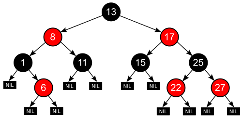
1.7.2. Red Black Tree
A Red Black Tree is a specialization of the Binary Search Tree, where the leaf nodes do not contain data.
- All nodes have an attribute flag of red or black
- The root is black
- All leaves (non-populated endpoints of the tree) are black
- All children of red items are black
- All paths from a given node to a descendent leaf (NIL) go through the same number of black nodes
2. Sorting algorithms
2.1. Insert Sort
Insertion sort is a simple sorting algorithm that is relatively efficient for small lists and mostly sorted lists. It works by taking elements from the list one by one and inserting them in their correct position into a new sorted list.
2.2. Selection Sort
Selection sort is an in-place comparison sort. It has O(n2) complexity, making it inefficient on large lists, and generally performs worse than the similar insertion sort. Selection sort is noted for its simplicity, and also has performance advantages over more complicated algorithms in certain situations.

2.3. Bubble Sort
Bubble sort is a simple sorting algorithm. The algorithm starts at the beginning of the data set. It compares the first two elements, and if the first is greater than the second, it swaps them. It continues doing this for each pair of adjacent elements to the end of the data set. It then starts again with the first two elements, repeating until no swaps have occurred on the last pass.
2.4. Quick Sort
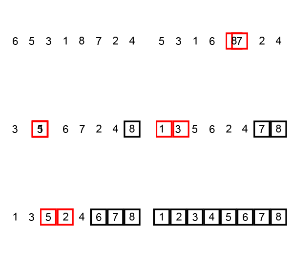
Quicksort is a divide and conquer algorithm which relies on a partition operation: to partition an array, an element called a pivot is selected. All elements smaller than the pivot are moved before it and all greater elements are moved after it. This can be done efficiently in linear time and in-place. The lesser and greater sublists are then recursively sorted. This yields average time complexity of O(n log n), with low overhead, and thus this is a popular algorithm. Efficient implementations of quicksort (with in-place partitioning) are typically unstable sorts and somewhat complex, but are among the fastest sorting algorithms in practice. Together with its modest O(log n) space usage, quicksort is one of the most popular sorting algorithms and is available in many standard programming libraries.
2.5. Heap Sort
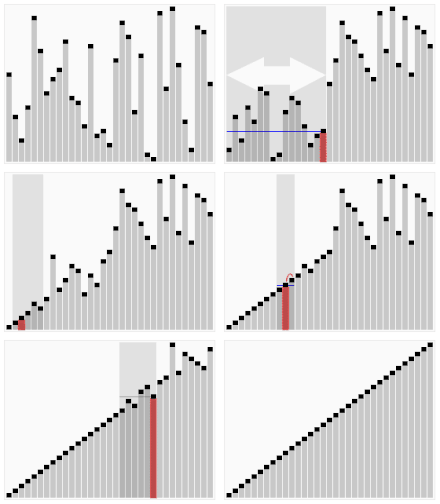
Heapsort is a much more efficient version of selection sort. It also works by determining the largest (or smallest) element of the list, placing that at the end (or beginning) of the list, then continuing with the rest of the list, but accomplishes this task efficiently by using a data structure called a heap, a special type of binary tree. Once the data list has been made into a heap, the root node is guaranteed to be the largest (or smallest) element. When it is removed and placed at the end of the list, the heap is rearranged so the largest element remaining moves to the root. Using the heap, finding the next largest element takes O(log n) time, instead of O(n) for a linear scan as in simple selection sort. This allows Heapsort to run in O(n log n) time, and this is also the worst case complexity.

2.6. Merge Sort
Merge sort takes advantage of the ease of merging already sorted lists into a new sorted list. It starts by comparing every two elements (i.e., 1 with 2, then 3 with 4…) and swapping them if the first should come after the second. It then merges each of the resulting lists of two into lists of four, then merges those lists of four, and so on; until at last two lists are merged into the final sorted list. Of the algorithms described here, this is the first that scales well to very large lists, because its worst-case running time is O(n log n). It is also easily applied to lists, not only arrays, as it only requires sequential access, not random access. However, it has additional O(n) space complexity, and involves a large number of copies in simple implementations.

3. Searching algorithms
Searching algorithms typically attempt to achieve efficiency within a defined problem domain, either in discrete or continuous data.
Searching algorithms are also highly dependent on the data types being stored and the data structure containing the data, and the order of the data within the structure.
3.1. Indexes
Indexes are used to quickly access data stored within a data set.
3.1.1. Forward Indexes
At a library, forward indexes are used in catalogs to help visitors find books based on a set of key words:
- Title
- Author
- Genre
- ISBN
These indexes however do very little to help the library visitor assess the content of the books on the shelves quickly.
Example of a Forward Index
| Document | Words |
|---|---|
| Document 1 | the,cow,says,moo |
| Document 2 | the,cat,and,the,hat |
| Document 3 | the,dish,ran,away,with,the,spoon |
Note: in the above forward index case the Words cannot be determined without first providing the Document
3.1.2. Inverted Index
In computer science, an inverted index (also referred to as a postings file or inverted file) is a database index storing a mapping from content, such as words or numbers, to its locations in a table, or in a document or a set of documents (named in contrast to a forward index, which maps from documents to content). The purpose of an inverted index is to allow fast full-text searches, at a cost of increased processing when a document is added to the database. The inverted file may be the database file itself, rather than its index. It is the most popular data structure used in document retrieval systems, used on a large scale for example in search engines. Additionally, several significant general-purpose mainframe-based database management systems have used inverted list architectures, including ADABAS, DATACOM/DB, and Model 204.
Example of an Inverted Index
| Word | Documents |
|---|---|
| the | Document 1, Document 3, Document 4, Document 5, Document 7 |
| cow | Document 2, Document 3, Document 4 |
| says | Document 5 |
| moo | Document 7 |
There are two main variants of inverted indexes:
- A record-level inverted index (or inverted file index or just inverted file) contains a list of references to documents for each word.
- A word-level inverted index (or full inverted index or inverted list) additionally contains the positions of each word within a document. The latter form offers more functionality (like phrase searches), but needs more processing power and space to be created.
3.1.3. Reverse Index
Reverse Indexes are used to reverse the digits or characters in a dictionary storage key to avoid contention in busy transactional data storage systems.
3.2. Database Pages
In relational databases, table data is typically stored in a set of sequential records spread over several Pages. When defining a table, the database configuration and table creation statements instruct how full each Page will be maintained. Pages which are mostly empty utilize excessive disk space, whereas pages which are mostly full suffer from fragmentation issues and modification delays.
Inside each Page, data is stored sequentially in contiguous blocks of memory.
Typically Pages are used to calculate hint statistics and metadata which aids as a high level search index to find the first item in each Page.
3.3. Search Algorithm concepts
3.3.1. Brute Force Search (No Knowledge)
A naive and simplistic exhaustive search where every element in a data structure is assessed for suitability against a search condition. This type of search is known to be exceptionally slow in unstructured and unsorted data.
3.3.2. Backward Induction Search
Backward induction is the process of reasoning backwards in time, from the end of a problem or situation, to determine a sequence of optimal actions. It proceeds by examining the last point at which a decision is to be made and then identifying what action would be most optimal at that moment. Using this information, one can then determine what to do at the second-to-last time of decision. This process continues backwards until one has determined the best action for every possible situation (i.e. for every possible information set) at every point in time.
- In the mathematical optimization method of dynamic programming, backward induction is one of the main methods for solving the Bellman equation.
- In game theory, backward induction is a method used to compute sub-game perfect equilibria in sequential games.
3.3.3. Heuristics Search (Partial Knowledge)
In mathematical optimization and computer science, heuristic (from Greek εὑρίσκω “I find, discover”) is a technique designed for solving a problem more quickly when classic methods are too slow, or for finding an approximate solution when classic methods fail to find any exact solution. This is achieved by trading optimality, completeness, accuracy, or precision for speed. In a way, it can be considered a shortcut.
A heuristic function, also called simply a heuristic, is a function that ranks alternatives in search algorithms at each branching step based on available information to decide which branch to follow. For example, it may approximate the exact solution.
3.3.4. Local Consistency and Constraint Propagation
In constraint satisfaction, local consistency conditions are properties of constraint satisfaction problems related to the consistency of subsets of variables or constraints. They can be used to reduce the search space and make the problem easier to solve. Various kinds of local consistency conditions are leveraged, including node consistency, arc consistency, and path consistency.
Every local consistency condition can be enforced by a transformation that changes the problem without changing its solutions. Such a transformation is called constraint propagation. Constraint propagation works by reducing domains of variables, strengthening constraints, or creating new ones. This leads to a reduction of the search space, making the problem easier to solve by some algorithms. Constraint propagation can also be used as an unsatisfiability checker, incomplete in general but complete in some particular cases.
3.4. Combinatorial Search
In computer science and artificial intelligence, combinatorial search studies search algorithms for solving instances of problems that are believed to be hard in general, by efficiently exploring the usually large solution space of these instances. Combinatorial search algorithms achieve this efficiency by reducing the effective size of the search space or employing heuristics
Lookahead constraints in combinatorial searches are used to limit the depth of search, as traditionally hard search domains quickly exhaust computing resources.
3.4.1. Alpha-Beta Pruning
Alpha–beta pruning is a search algorithm that seeks to decrease the number of nodes that are evaluated by the minimax algorithm in its search tree. It is an adversarial search algorithm used commonly for machine playing of two-player games (Tic-tac-toe, Chess, Go, etc.). It stops evaluating a move when at least one possibility has been found that proves the move to be worse than a previously examined move. Such moves need not be evaluated further. When applied to a standard minimax tree, it returns the same move as minimax would, but prunes away branches that cannot possibly influence the final decision.
3.4.2. Branch and Bound
Branch and bound (BB, B&B, or BnB) is an algorithm design paradigm for discrete and combinatorial optimization problems, as well as mathematical optimization. A branch-and-bound algorithm consists of a systematic enumeration of candidate solutions by means of state space search: the set of candidate solutions is thought of as forming a rooted tree with the full set at the root. The algorithm explores branches of this tree, which represent subsets of the solution set. Before enumerating the candidate solutions of a branch, the branch is checked against upper and lower estimated bounds on the optimal solution, and is discarded if it cannot produce a better solution than the best one found so far by the algorithm.
The algorithm depends on efficient estimation of the lower and upper bounds of regions/branches of the search space. If no bounds are available, the algorithm degenerates to an exhaustive search.
3.4.3. MinMax
Minimax (sometimes MinMax, MM] or saddle point) is a decision rule used in artificial intelligence, decision theory, game theory, statistics, and philosophy for minimizing the possible loss for a worst case (maximum loss) scenario. When dealing with gains, it is referred to as “maximin”—to maximize the minimum gain. Originally formulated for n-player zero-sum game theory, covering both the cases where players take alternate moves and those where they make simultaneous moves, it has also been extended to more complex games and to general decision-making in the presence of uncertainty.
4. Graphs
4.1. Graph Search
4.1.1. Breadth First Search
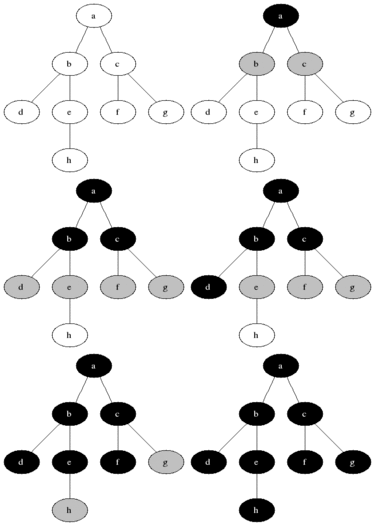
Breadth-first search (BFS) is an algorithm for traversing or searching tree or graph data structures. It starts at the tree root (or some arbitrary node of a graph, sometimes referred to as a ‘search key’), and explores all of the neighbor nodes at the present depth prior to moving on to the nodes at the next depth level.
Breadth-first search is excellent at reducing the problem domain scope, when combined with pruning.
Pseudocode
procedure BFS(G, root) is
  let Q be a queue
  label root as discovered
  Q.enqueue(root)
  while Q is not empty do
    v := Q.dequeue()
    if v is the goal then
      return v
    for all edges from v to w in G.adjacentEdges(v) do
      if w is not labeled as discovered then
        label w as discovered
        Q.enqueue(w)
4.1.2. Depth First Search
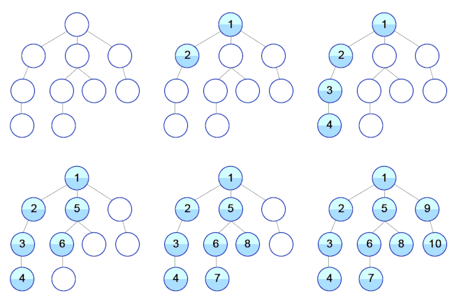
Depth-first search (DFS) is an algorithm for traversing or searching tree or graph data structures. The algorithm starts at the root node (selecting some arbitrary node as the root node in the case of a graph) and explores as far as possible along each branch before backtracking.
Due to the nature of exhaustive evaluation of a branch before backtracking, it is a natural search algorithm which pairs with recursive functions.
procedure DFS_iterative(G, v) is
    let S be a stack
    S.push(v)
    while S is not empty do
        v = S.pop()
        if v is not labeled as discovered then
            label v as discovered
            for all edges from v to w in G.adjacentEdges(v) do
                S.push(w)
4.1.3. A* Star Search
A* is an informed search algorithm, or a best-first search, meaning that it is formulated in terms of weighted graphs: starting from a specific starting node of a graph, it aims to find a path to the given goal node having the smallest cost (least distance travelled, shortest time, etc.). It does this by maintaining a tree of paths originating at the start node and extending those paths one edge at a time until its termination criterion is satisfied.

Further Reading for Goal Oriented Action Planning
5. Divide and Conquer vs. Dynamic Programming
5.1. Optimal Substructure
A problem is said to have optimal substructure if an optimal solution can be constructed from optimal solutions of its subproblem

5.2. Overlapping Sub-problems
A problem is said to have overlapping sub-problems if the problem can be broken down into sub-problems which are reused several times or a recursive algorithm for the problem solves the same subproblem over and over rather than always generating new sub-problems.
5.3. Divide and Conquer
Divide and Conquer algorithms solve a specific high level problem by dividing the problem into simpler independent sub-problems, then solving those, before combining the result to achieve the solution to the high level problem.
Typically, Divide and Conquer is used to determine the optimal solution to a problem.
The conditions for a problem to be solvable by divide and conquer are:
- Divisibility of the problem, into sub-problems
- Optimal solutions achievable for sub-problems
- The sub-problems must not overlap.
Therefore, we say Divide and Conquer algorithms:
- Must have Optimal Substructure
- Must not have Overlapping Sub-problems
Traditional examples of Divide and Conquer include:
- Quick Sort
- Merge Sort
5.4. Dynamic Programming
Dynamic Programming, like Divide and Conquer algorithms, pertains to the division of a problem into smaller sub-problems, to derive the solution to a complex problem.
However, unlike Divide and Conquer algorithms, Dynamic Programming algorithms:
- Must have Optimal Substructure
- Must have Overlapping Sub-problems
Traditional examples of Dynamic Programming algorithms include:
- Tower of Hanoi algorithm
- Fibonacci algorithm
Using Memoization, typically a table can be used to store the results of dynamic programming sub-problem solutions to quickly construct solutions to complex Dynamic Programming problems.
6. Genetic Algorithms
Genetic Algorithms are derived from traditional biological processes of genetic mixing, through instruction and variable selection, crossover, and mutation. Due to their ability to solve traditionally hard problems, without using human deductive reasoning, they are often used when other techniques have failed to achieve an appropriate solution. Conceptually, in this domain, programs are able to write themselves, as a satisfactory measure is inbuilt to determine when a solution achieves a goal. In addition, genetic algorithms are only really practical when operating in parallel with a pool simultaneous algorithms competing to solve the solution.
7. Constraint Satisfaction Problems
Constraint Satisfaction Problems (CSPs) are a broad strategy to define the conditions under which a problem can be deemed solved.
- Variables - The contextual players of the problem,
- Domains - The contextual options which govern the players
- Constraints - The contextual limitations placed upon the players and domain, which must be satisfied to achieve a solution to the problem
7.1. CSP Example using Sudoku
In classic sudoku, the objective is to fill a 9×9 grid with digits so that each column, each row, and each of the nine 3×3 subgrids that compose the grid (also called “boxes”, “blocks”, or “regions”) contain all of the digits from 1 to 9. The puzzle setter provides a partially completed grid, which for a well-posed puzzle has a single solution.
Variables
- The 81 cells within the 9x9 grid Domain
- The numbers from 1 to 9, and empty
- The 9 rows
- The 9 columns
- The 9 3x3 sub-grids Constraints
- That each row must contain the numbers 1 through 9
- That each column must contain the numbers 1 through 9
- That each 3x3 sub-grid must contain the numbers 1 through 9
- That any cell already containing a value in the supplied partially completed grid, is fixed
- That all 81 cells must contain a value (redundant as covered already by the above constraints)
Note: It is intentional to word the constraints all in positive language, however it is possible to write the constraints in negative constraints also. By writing them all as either positive conditions, or negative conditions, the implementation is more consistent.
7.2. CSP solutions
The primary problem is finding the state of a set of variables within the domains which satisfy the constraints.
Options to tackle CSPs typically require a couple of core features.
- Data structures to store the lists of variables, domains (and probably constraints also)
- Operations which iterate over possible solutions, but stop when solution is solved
- Operations which evaluate each and all of the constraints, for a given set of variables and domain
- Optimizations
- Operations which recognize when a path to seek a solution is a dead end (Back tracking)
- Operations which can forward search for easy solutions when nearly complete (Look ahead)
8. Clustering Algorithms
Clustering algorithms attempt to detect similarity between values within data sets, such that automated grouping can be achieved. Clustering algorithms are used extensively in machine learning, particularly in unsupervised learning or data set inspection.
Clustering algorithm are useful for classifying groups of points, and also for finding outliers in the data set.
8.1. K-Means Clustering
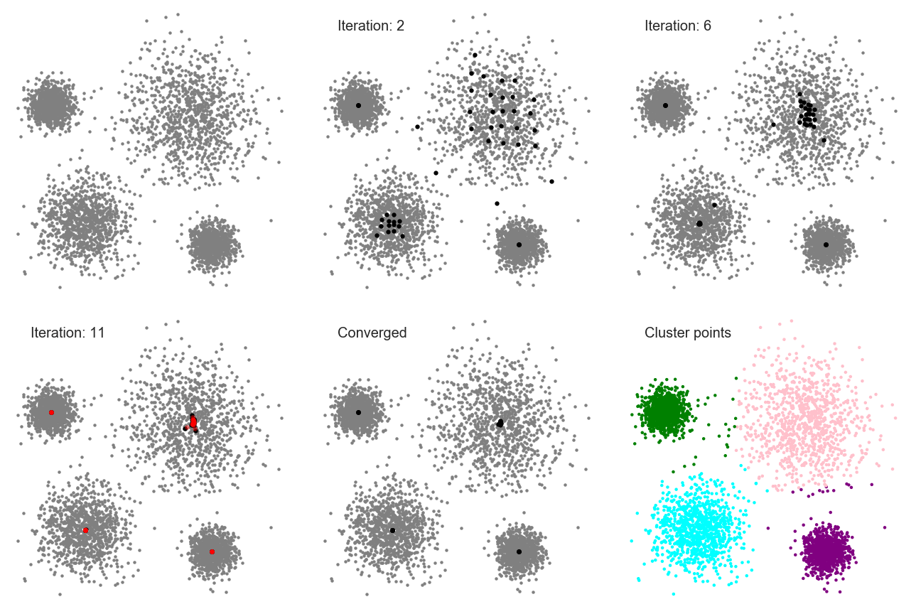
K-Means is one of the most trivial clustering algorithms and is easy to implement.

- Select K random points as centroids in the data set range
- For each data set point, assign the data set point to the nearest centroid (using the squared Euclidean distance)
- Update the centroid position, such that the new position is in the mean of the assigned data points
- Repeat steps 2 and 3 until convergence occurs and the centroids no longer move
Issues:
- Not guaranteed to find optimum solution
- Performance dependent on
- the number of K
- the number of data set points
- initial position of starting points
- the rate of movement into convergence locations
- the detection of convergence
8.2. K-Nearest Neighbor Clustering
- Load the data
- Initialize K to your chosen number of neighbors
- For each example in the data
- Calculate the distance between the query example and the current example from the data. i.e. Distance each point between neighbors.
- Add the distance and the index of the example to an ordered collection
- Sort the ordered collection of distances and indices from smallest to largest (in ascending order) by the distances
- Pick the first K entries from the sorted collection
- Get the labels of the selected K entries
- If regression, return the mean of the K labels
- If classification, return the mode of the K labels
Issues:
- Slow as the number of points increases
- Improvements can be made by limiting the range of search to find neighbors
8.3. Mean Shift
Means Shift algorithm is used to achieve clustering in a non-circular solution.
When using means shift, each data point slowly progresses over a gradient toward local means.

- First, calculate the Kernel Density Estimate for the data points.
- Shift each point toward the local maxima, from the KDE.
Benefits:
- Highly resilient to outliers in the data set
- Great at deducing the number of clusters
Issues:
- Not guaranteed to result in an optimum result
- Calculating the KDE can be costly
8.4. Density Based Spatial Clustering (DBSCAN)
8.5. Expectation Maximization Clustering using Gaussian Mixture Models (GMMs)

8.6. Agglomerative Hierarchical Clustering
9. Compression Algorithms
Compression algorithms are described as being lossy or lossless:
- Lossy compression results in the loss of detail, and permanent degradation of the source data, and is therefore a one-way operation
- Lossless compression results in the complete reconstruction of source data, and is therefore a reversible operation
9.1. Image and Video compression
Image compression techniques typically utilize lossy approaches, as users are typically not concerned about the visual loss of detail, when it is moderately applied.
Popular image compression algorithms include:
- JPEG
- GIF
- TIFF
- H.263 and H.264 / MPEG-4
9.2. Audio compression
Audio compression techniques typically utilize lossy approaches to remove artifacts which remove aspects outside the typical human-audible range.
Popular audio compression algorithms include:
9.3. Text and Binary data compression
Text compression techniques require lossless approaches, as the degradation of text is typically undesirable, resulting in the loss of meaning of the text.
Binary data is considered to require complete reconstruction, via decompression, and therefore requires a lossless techniques.
Popular compression algorithms include:
- Lempel-Ziv (LZ) and Lempel-Ziv-Welch LZW
- GZip which uses Huffman coding and LZ77
9.3.1. Huffman coding
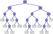
A Huffman code is a particular type of optimal prefix code that is commonly used for lossless data compression. The Huffman coding algorithm is used to get Huffman codes.
The output from Huffman’s algorithm can be viewed as a variable-length code table for encoding a source symbol (such as a character in a file). The algorithm derives this table from the estimated probability or frequency of occurrence (weight) for each possible value of the source symbol.
9.3.1.1. Huffman Tree
9.3.1.2. Construction of a Huffman Tree

9.3.1.3 Huffman Code table
| Input (A, W) | Symbol (ai) | a | b | c | d | e | Sum |
| Weights (wi) | 0.10 | 0.15 | 0.30 | 0.16 | 0.29 | = 1 | |
| Output | C | Codewords (ci) | 010 | 011 | 11 | 00 | 10 |
| Codeword length (in bits) (li) | 3 | 3 | 2 | 2 | 2 | ||
| Contribution to weighted path length (li wi ) | 0.30 | 0.45 | 0.60 | 0.32 | 0.58 | L(C) = 2.25 | |
| Optimality | Probability budget (2−li) | 1/8 | 1/8 | 1/4 | 1/4 | 1/4 | = 1.00 |
| Information content (in bits) (−log2 wi) ≈ | 3.32 | 2.74 | 1.74 | 2.64 | 1.79 | ||
| Contribution to entropy(−wi log2 wi) | 0.332 | 0.411 | 0.521 | 0.423 | 0.518 | H(A) = 2.205 |
where:
-
Weights are typically proportional to probabilities of the symbol
-
Information content h
-
Entropy


